How To Find Missing Data Using Vlookup
Insert the formula in IF ISERROR VLOOKUP A2B2B10011FALSEFALSETRUE the formula bar. For VLOOKUP this first argument is the value that you want to find.
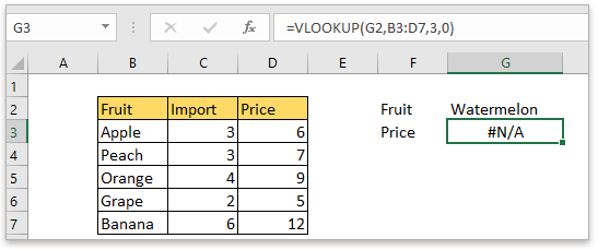
Lookup To Return Default Value If Not Found Match Value In Excel
So my final stage of the formula is to simply drag the formula to row 20 to allow Excel to see what rows up to and including 20 are missing.

How to find missing data using vlookup. Compare Two Columns Using VLOOKUP and Find Differences Missing Data Points While in the above example we checked whether the data in one column was there in another column or not. Press Enter to assign the formula to C2. You can check if the values in column A exist in column B using VLOOKUP.
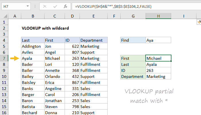
If you want to retrieve employee information from a table and the table contains a unique id to the left of the information you want to retrieve you can easily do so with the VLOOKUP function. You can use behavior directly inside an IF statement to mark values that have a zero count ie. If the first VLOOKUP does not find a match on the first sheet search in the next sheet and so on.
A step-by-step guide on Amazon - httpsamznto2qokYzjThis video tutorial provides a walk through on how to merge data contained wi. Keep default value in values with dropdown list. Click Home in ribbon click Conditional Formatting in Styles group.
Combining 2 Spreadsheets Locate where you want the data to go. 2 Check Each row from the Based on section. VLOOKUP What you want to look up where you want to look for it the column number in the range containing the value to return return an Approximate or Exact match indicated as 1TRUE or 0FALSE.
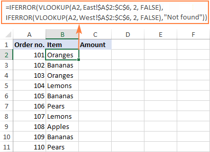
The idea is to nest several IFERROR functions to check multiple worksheets one by one. Then the matched values will give us the confirmation using the IF function. In Duplicate Values dialog select Unique in dropdown list.
That way we could use the function to reference the invoice number from his list and check. The third argument is the column in that range of cells that contains the value that you seek. In place of MATCH function VLOOKUP function is used here with ISNA function to find the missing values.
In the example shown the formula in G6 is. In Conditional Formatting dropdown list select Highlight Cells Rules-Duplicate Values. The following figure shows the results with VLOOKUP function with the formula mentioned in it.
Select the first blank cell besides Fruit List 2 type Missing in Fruit List 1 as column header next enter the formula IF ISERROR VLOOKUP A2Fruit List 1A2A221FALSEA2 into the second blank cell and drag the Fill Handle to the range as you need. You can also use the same concept to compare two columns using the VLOOKUP function and find missing data. A vertical lookup is used to look for specific data in the first column of a data table.
1 Select the data list in Names-1 sheet under the Find values in and then select the data from Names-2 sheet under the According to. Compare Two Columns to Find Missing Value by Conditional Formatting. Select List A and List B.
3 Choose Same Values from the Find section. We will construct a formula out of it. VLOOKUP returns a NA error if a value is not found from the list.
If the result of the VLOOKUP Function is not NA and the row number is found then we simply get Excel to return a blank cell using the double quotes. In its simplest form the VLOOKUP function says. IFCOUNTIF list F6 OKMissing where list is.
The second argument is the range of cells C2-E7 in which to search for the value you want to find. The IF function returns the confirmation using the values Is there Missing. In the example shown the VLOOKUP formula looks like this.
Well walk through each part of the formula. 4 Then you can choose background color or font color for the same names which are in both sheets as you need. Click that cell only once.
When you need to look up between more than two sheets the easiest solution is to use VLOOKUP in combination with IFERROR. Select vLookup Excels vLookup wizard will pop up. Missing values can also be found with the help of VLOOKUP function.
This argument can be a cell reference or a fixed value such as smith or 21000. Values that are missing. If no cells meet criteria COUNTIF returns zero.
Once it finds the row that holds the data you are looking for it then bounces across to another column in the same table of data and returns information from it. Dragging The Excel Formula. At the top go to the Formulas tab and click Lookup Reference.
We decided to insert the VLOOKUP function in Guys workbook. Firstly the lookup value is searched in the particular column of the table array. Select cell C2 by clicking on it.

Finding Missing Items With Vlookup Solution Next Video Shown In Description Youtube

How To Use Vlookup Vlookup Exact Match Vlookup Approximate Match Exce Tutorial Microsoft Excel Excel
![]()
How To Vlookup To Return Blank Or Specific Value Instead Of 0 Or N A In Excel

Excel Formula Faster Vlookup With 2 Vlookups Exceljet

Excel Vlookup With Missing Data Super User
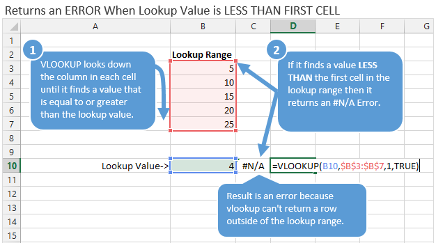
Vlookup To Find The Closest Match Last Argument True

Change Text 3 Methods Into Upper Case Lower Case Or Proper Case In Exc Lowercase A Upper Case Change Text
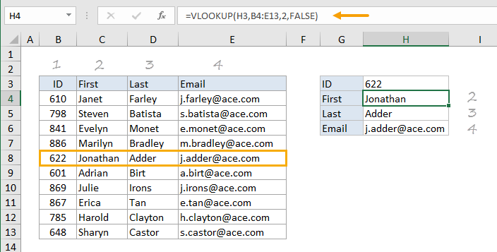
How To Use The Excel Vlookup Function Exceljet

Excel Formula Find Missing Values Exceljet
![]()
How To Vlookup To Return Blank Or Specific Value Instead Of 0 Or N A In Excel
Vlookup Example 5 Lookup Table Computer Technology Function

How To Find Missing Items In A Column With Consecutive Numbers In Excel Worksheet Excel Excel Formula Column

How To Use Vlookup With An Excel Spreadsheet Excel Spreadsheets Spreadsheet Excel Formula
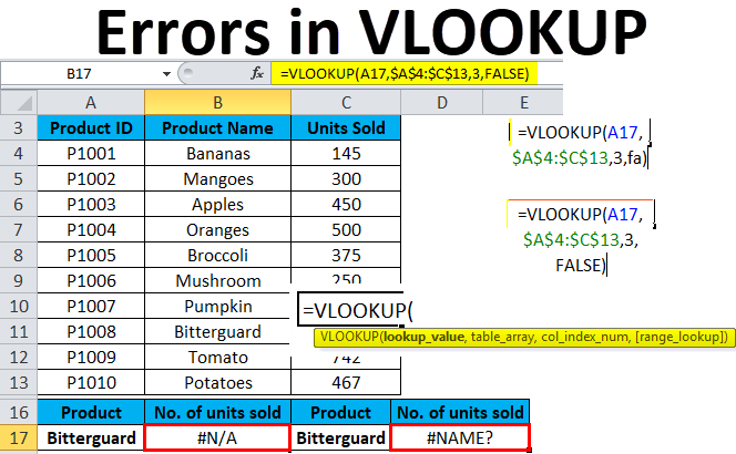
Vlookup Errors Examples How To Fix Errors In Vlookup

Excel Vlookup Function Vlookup Excel Microsoft Excel Excel Tutorials

Excel Formula Vlookup Without N A Error Exceljet
How To Use The Excel Vlookup Function Exceljet
Vlookup Across Multiple Sheets In Excel With Examples

How To Troubleshoot Vlookup Errors In Excel